Big O notation and the Bachmann-Landau family

Most of us, software engineers, are familiar with (or, at least, have heard of) the well-known "Big O" notation (O-notation for short). The reasons are diverse. O-notation is a concept that arises frequently in technical interviews, so it is likely that we come across O-notation at some point in our careers. We can also simply like theoretical computer science or work in a domain where the design and analysis of algorithms is relevant.
O-notation allows you to characterize the asymptotic efficiency of algorithms. Using O-notation, you can describe how the running time and the required memory of an algorithm increase with the size of the input, as the size of the input grows without bound.
For example, you can say that the worst-case running time of selection sort is O(n²). Informally, this means that the running time of selection sort is bounded from above by a quadratic function of n, where n is the size of the input.
The focus of this post is not on explaining O-notation, however. Here, I assume that you have basic understanding of O-notation and I focus on an aspect of this notation that is arguably less well-known.
Did you know that O-notation is part of a wider family of related notations?
This family is called: the Bachmann-Landau notation.
There are invaluable resources that cover the Bachmann-Landau notation in detail. For example, in these books:
Introduction to Algorithms (3rd edition). Cormen, Thomas H.; Leiserson, Charles E.; Rivest, Ronald L.; Stein, Clifford. The MIT Press (2009).
The Algorithm Design Manual (2nd edition). Skiena, Steven S. Springer (2008).
You will find formal definitions, detailed examples, exercises, and even other notations that I do not cover here.
In this post, I focus on three notations of the Bachmann-Landau family:
- O (Big O)
- Ω (Big Omega)
- ϴ (Big Theta)
My description of these notations is deliberately informal. My goal is just to give you a feel for what these notations are about and why they are useful.
A running example
Through this post, I use Quicksort as an example.
Quicksort is a divide-and-conquer comparison-based sorting algorithm. Even though it has a slow worst-case running time, it is often the best practical choice for sorting because it is remarkably efficient on average.
For this post, let's assume a Quicksort implementation that always takes a quadratic number of steps in the worst-case. And let's also assume that n represents the size of the input, which, in this case, is the size of the input array.
A general view of the Bachmann-Landau notation
In general terms, the asymptotic notations of the Bachmann-Landau family are used to compare functions.
You can express the running time of an algorithm as a function f(n), and, for example, you can say that f(n) = O(g(n)). This means that, for all sufficiently large values of n, the value f(n) is less than or equal to g(n) to within a constant factor.
This comparison-centric point of view is important because the different notations of the Bachmann-Landau family give you the different comparison operators: ≤, ≥ and =.
O-notation
In simple and informal terms:
O-notation gives you a rough notion of less-than-or-equal-to (≤).
In the Quicksort example, you can say the worst-case running time of Quicksort is O(n²).
This means that the worst-case of Quicksort takes at most a quadratic number of steps.
You could also say that the worst-case of Quicksort is O(n³) because O establishes only an upper bound.
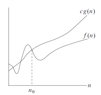
If you write that f(n) = O(g(n)), then the function g(n) is an asymptotically upper bound for f(n).

Observe in the figure (taken from the "Introduction to Algorithms" book) that we do not care about small values of n (that is, anything smaller than n₀). After all, we do not care whether an algorithm sorts 5 items faster than another. We care about large values of n.
Observe also that the upper bound is not actually g(n). It is g(n) multiplied by some positive constant c. However, O-notation typically ignores such multiplicative constants.
Ω-notation
While O-notation allows you to express upper bounds, Ω-notation gives you the opposite:
Ω-notation gives you a rough notion of greater-than-or-equal-to (≥).
In the Quicksort example, you can say that the worst-case of Quicksort is Ω(n²).
This means that, in its worst-case, Quicksort takes at least a quadratic number of steps.
You could also say that the worst-case of Quicksort is Ω(n) because Ω establishes only a lower bound.
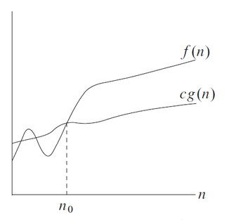
If you write that f(n) = Ω(g(n)), then the function g(n) is an asymptotically lower bound for f(n).

ϴ-notation
Unlike O and Ω notations:
ϴ-notation gives you a rough notion of equality (=).
For example, you can say that the worst-case of Quicksort is ϴ(n²).
This means that the worst-case of Quicksort takes exactly a quadratic number of steps.
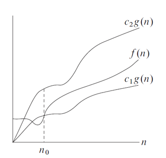
ϴ is a stronger notion than O and Ω because it establishes both an upper and a lower bound.
Therefore, if you write f(n) = ϴ(g(n)), then both f(n) = Ω(g(n)) and f(n) = O(g(n)) hold.
If you write that f(n) = ϴ(g(n)), then the function g(n) is an asymptotically tight bound for f(n).

Conclusion
There are notable exceptions, but it is likely that you will not use Bachmann-Landau notation as part of your daily job. At least, that’s my experience. But, even then, becoming familiar with it (and with the analysis of algorithms in general) is far from useless. Once you get the hang of it, you start considering trade-offs that never existed for you before. You start thinking about what solution is faster for your problem and what implementation is more memory-efficient.
You will start asking yourself: can I do better?
You will still give priority to writing code that is clean and can be maintained easily. But, you will not forget that, after making it work and making it right, you may need to make it fast.


